Concluded·23 Jul 2026 · 12 min read
TimescaleDB as a plant historian: a 40-million-row load test on a home lab
TimescaleDB · Docker · Grafana · PostgreSQL
Every plant that runs long enough grows a data problem before it grows a
data strategy. Tags pile up — a temperature probe here, a flow meter there —
each one sampled every few seconds, every one of them forever. A year later
someone in the front office asks a reasonable question: what was the average
outlet temperature, per line, per month, for the last three years? And on
most sites the answer is a spreadsheet exported by hand, because the
"historian" is a folder of CSV files or a SQL table nobody dares run a
GROUP BY against.
A proper historian solves exactly this. It swallows high-frequency time-stamped data cheaply, keeps years of it without bankrupting the disk, and answers time-bucketed questions fast enough that a monthly report is a query, not a project. TimescaleDB is PostgreSQL taught to do this — the same database your team already runs, extended with hypertables, native compression, and continuous aggregates.
I wanted to know how much of that pitch survives contact with real data, so I ran it. Not a vendor benchmark — a box in my own rack, three years of one-minute readings, plain Postgres in one table and a hypertable in another, side by side. But first, the part worth understanding before the benchmark: why a hypertable, and not just a table.
First, what a historian does to a database
A plant historian has a very particular shape, and it's worth naming before picking a tool for it:
- It's write-heavy. Every sensor writes on its own clock — every second, every few seconds — and never stops. Hundreds of tags become millions of new rows a day. The database spends most of its life inserting.
- It's append-only and time-ordered. New data is almost always now. You rarely update or delete an old reading; you keep adding to the front.
- It's read by time. Nobody asks for "row number 8,000,000." They ask for "the last 24 hours," "last month per line," "this shift versus the same shift last year." Every read is a time range.
A regular Postgres table can absolutely hold this. The trouble starts as it grows. It's one big pile of rows behind one big index, so two things go wrong at once: every insert has to update that ever-growing index, so writes get slower as history piles up; and because it's a single pile, "the last 24 hours" still makes the database reason about all three years to find them — unless you hand-build and maintain indexes, which then slow the writes down further. Write-heavy and read-by-time pull against each other on a plain table.
Regular table vs hypertable, in plain terms
A hypertable is TimescaleDB's answer, and the important part is what
doesn't change: from where you sit it's still one table. Same CREATE TABLE,
same INSERT, same SELECT, same Postgres. You point your historian at it
exactly as before.
What changes is underneath. TimescaleDB automatically slices the table into many small tables — one chunk per time window (a week, in this test) — and routes each row to the right chunk by its timestamp. You never manage the chunks; you query the one table and it handles the rest.
That single choice — slice by time — is what makes it fit a historian:
- Writes stay in a small, hot chunk. New readings only ever land in the newest chunk, small enough to sit in memory with its index. Inserts don't slow down as the years accumulate, because they never touch the old chunks.
- Reads skip what they don't need. A "last 24 hours" query looks at one chunk and ignores the other 156 — chunk exclusion. You get time-range speed without hand-building indexes.
- Old data compresses without disturbing new writes. Because history is already sliced, each old chunk can be squeezed into compact columnar form while the hot chunk keeps taking writes at full speed.
Why this, and not something else
- Versus a plain Postgres table: writes that don't degrade over time, free time-range performance, and compression you can still query — the three things a plain table can't give you at once.
- Versus a dedicated time-series database (InfluxDB and friends): those are fast too, but they're a second system to learn, run, back up, and join against. TimescaleDB is just Postgres, so asset tables, work orders, and sensor history live in one database you already operate.
- Versus a closed historian appliance: open source, on-prem when the plant demands it, no per-tag licensing.
For any plant that already runs Postgres somewhere in the building, the hypertable is the lowest-friction way to make sensor history fast. That's why I tested it before recommending it — the rest of this piece is that test.
The box: Ubuntu, then Docker
The host is an Ubuntu-family Linux container. If you're starting from bare metal, install Ubuntu Server 24.04 first; Canonical's own walkthrough is the one I keep sending people to — Install Ubuntu Server. On a machine that already runs Linux you can skip straight ahead.
Then Docker. Don't hand-roll it — use Docker's own apt repository, which is the only install path they support and keep current. The official guide is short and correct: Install Docker Engine on Ubuntu. Two commands afterwards and you're set:
# verify the engine is alive
sudo docker run hello-world
# let your user drive docker without sudo
sudo usermod -aG docker $USER && newgrp docker
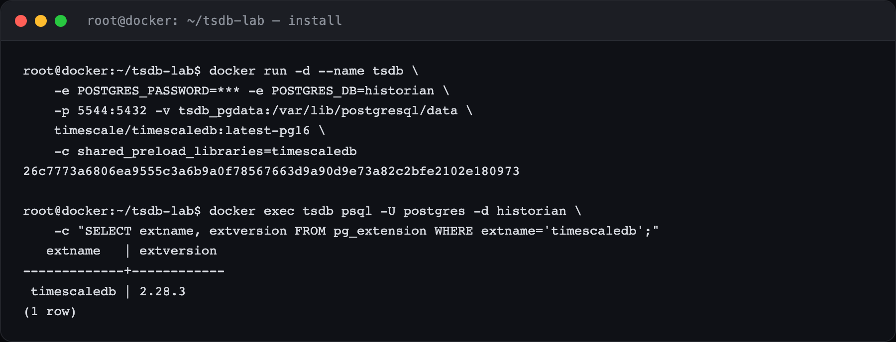
TimescaleDB in one container
TimescaleDB ships a ready image with the extension already compiled against
PostgreSQL. One docker run gives you a working historian — a named volume
keeps the data across restarts, and host port 5544 maps to Postgres inside:
docker run -d --name tsdb \
  -e POSTGRES_PASSWORD=*** \
  -e POSTGRES_DB=historian \
  -p 5544:5432 \
  -v tsdb_pgdata:/var/lib/postgresql/data \
  timescale/timescaledb:latest-pg16 \
  -c shared_preload_libraries=timescaledb
That's the entire installation. Confirm the extension loaded and you have a time-series database:
Two tables, one difference
You've seen the idea; here it is in SQL. To keep the comparison honest, both
tables get the same schema and the same rows — one plain, one a hypertable.
The only line that differs is create_hypertable, which turns the second one
into time-sliced chunks:
CREATE TABLE readings_plain (
  time        timestamptz NOT NULL,
  device_id   int         NOT NULL,
  temperature double precision,   -- degrees C
  pressure    double precision,   -- bar
  vibration   double precision,   -- mm/s
  flow        double precision    -- m3/h
);

CREATE TABLE readings_hyper (LIKE readings_plain);
SELECT create_hypertable('readings_hyper', 'time',
       chunk_time_interval => interval '7 days');
Mimicking three years of a plant
Real historian data isn't random noise. A temperature probe traces a smooth
curve: a slow annual season riding under a daily heat-of-the-day cycle, and —
this part matters — reported at limited precision. A real transmitter sends
23.4 °C, not 23.4187625, and holds that value for minutes at a time. I
generated exactly that, deterministically, rounded to sensor precision, so
both tables receive byte-for-byte identical values:
INSERT INTO readings_hyper
SELECT
  t,
  d,
  round((22 + 12*sin(2*pi()*extract(epoch FROM t)/31557600.0)  -- annual season
            +  6*sin(2*pi()*extract(epoch FROM t)/86400.0)     -- day / night
            +  (d % 7))::numeric, 1),                           -- to 0.1 C
  /* pressure, vibration, flow … */
FROM generate_series(
       timestamptz '2023-01-01',
       timestamptz '2025-12-31 23:59',
       interval '1 minute') AS t
CROSS JOIN generate_series(1, 25) AS d;
Twenty-five probes, one reading a minute, three full years: 39,456,000 rows in each table. A small plant's worth of history — and enough to make the difference between "table" and "hypertable" obvious.
Result 1 — ingest
Loading the identical 39.5 million rows, one plain INSERT … SELECT each:
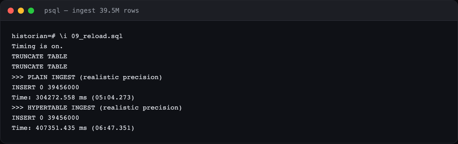
| Target | Load time | Rate |
|---|---|---|
| Plain PostgreSQL table | 5 min 04 s | ~130,000 rows/s |
| TimescaleDB hypertable | 6 min 47 s | ~97,000 rows/s |
Be honest about this: the hypertable is ~35% slower to ingest. Routing
every row to the right weekly chunk costs something. In production you'd claw
most of it back with COPY and batched writes, but the headline stands —
plain Postgres wins the write race. Everything after this, the hypertable
wins, and wins big.
Result 2 — the long data plane, compressed
This is where a historian earns its name. Three years of raw rows take real disk. Turn on TimescaleDB's native columnar compression — segment by device, order by time — and each weekly chunk is rewritten into compressed columnar form:
ALTER TABLE readings_hyper SET (
  timescaledb.compress,
  timescaledb.compress_segmentby = 'device_id',
  timescaledb.compress_orderby   = 'time DESC'
);
SELECT compress_chunk(c) FROM show_chunks('readings_hyper') c;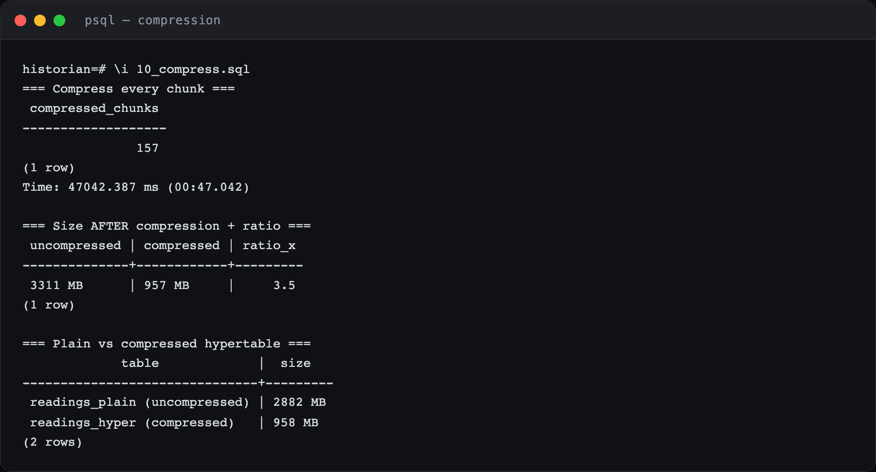
| Table | On disk |
|---|---|
| Plain PostgreSQL | 2882 MB |
| Hypertable, uncompressed | 3311 MB |
| Hypertable, compressed | 957 MB |
The hypertable started larger than plain Postgres — the per-chunk index overhead — and compression turned that into 3× smaller than plain, a 3.5× reduction against its own uncompressed size. And this is not an archive tier: the compressed minute-data is still fully queryable, in place. You don't down-sample or ship anything to cold storage to get it back.
Result 3 — time_bucket, and the report that used to hurt
The question that started this piece — average temperature per probe per
month, across three years — is a GROUP BY over 39.5 million rows. Plain
Postgres reaches for date_trunc; TimescaleDB gives you time_bucket, which
bins on any interval and understands the partitioning underneath:
-- plain
SELECT device_id, date_trunc('month', time) AS month, avg(temperature)
FROM readings_plain GROUP BY device_id, month;

-- hypertable
SELECT device_id, time_bucket('1 month', time) AS month, avg(temperature)
FROM readings_hyper GROUP BY device_id, month;
Both still read every row. The real fix is a continuous aggregate — a materialised, incrementally-refreshed rollup. Define the daily average once and TimescaleDB keeps it current as new data lands:
CREATE MATERIALIZED VIEW temp_daily
WITH (timescaledb.continuous) AS
SELECT device_id, time_bucket('1 day', time) AS day,
       avg(temperature) AS avg_t, max(temperature) AS max_t, min(temperature) AS min_t
FROM readings_hyper
GROUP BY device_id, day;
Now the three-year monthly report reads from 27,400 pre-aggregated daily
rows (4.3 MB) instead of 39.5 million raw ones. Here is the same report
down all three paths, measured with EXPLAIN ANALYZE:
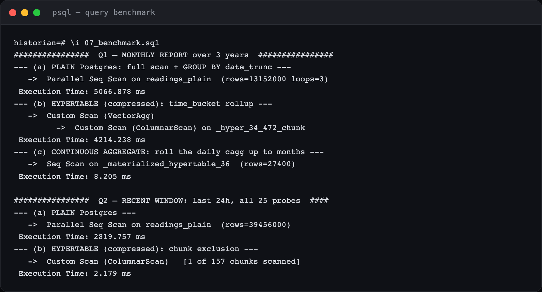
| Monthly report, 3 years | Rows scanned | Execution time |
|---|---|---|
Plain Postgres (date_trunc) | 39,456,000 | 5067 ms |
Hypertable (time_bucket, compressed) | 39,456,000 | 4214 ms |
| Continuous aggregate | 27,400 | 8.2 ms |
That report went from five seconds to eight milliseconds — about 600×. And a "what happened in the last day" query, the bread and butter of any control room, is even starker. Because the hypertable is partitioned by time, it reads only the one chunk that holds recent data and skips the other 156 entirely:
| Last-24h detail, 25 probes | Rows scanned | Execution time |
|---|---|---|
| Plain Postgres | 39,456,000 (full scan) | 2820 ms |
| Hypertable (chunk exclusion) | 1 of 157 chunks | 2.2 ms |
Nearly 1300× faster, from the same data, with no extra indexes — just the time partitioning doing its job.
Seeing it — Grafana on the same data
Numbers convince engineers; pictures convince everyone else. I pointed Grafana
at the historian (PostgreSQL data source, the tsdb container as host) and
built one dashboard straight off the tables and the continuous aggregate.
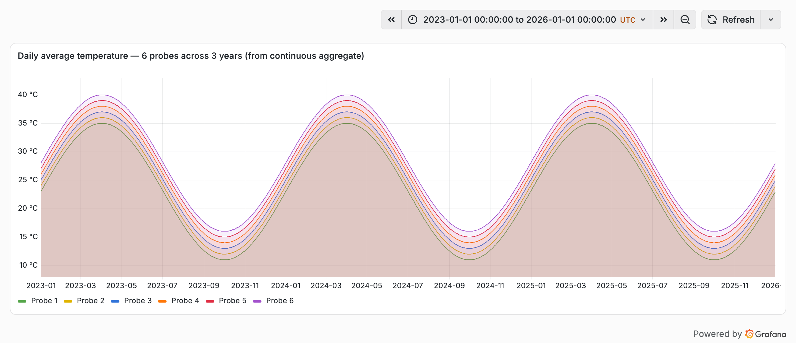
The three-year daily average, six probes, drawn from the continuous aggregate. The annual season is unmistakable — three summers, three winters:
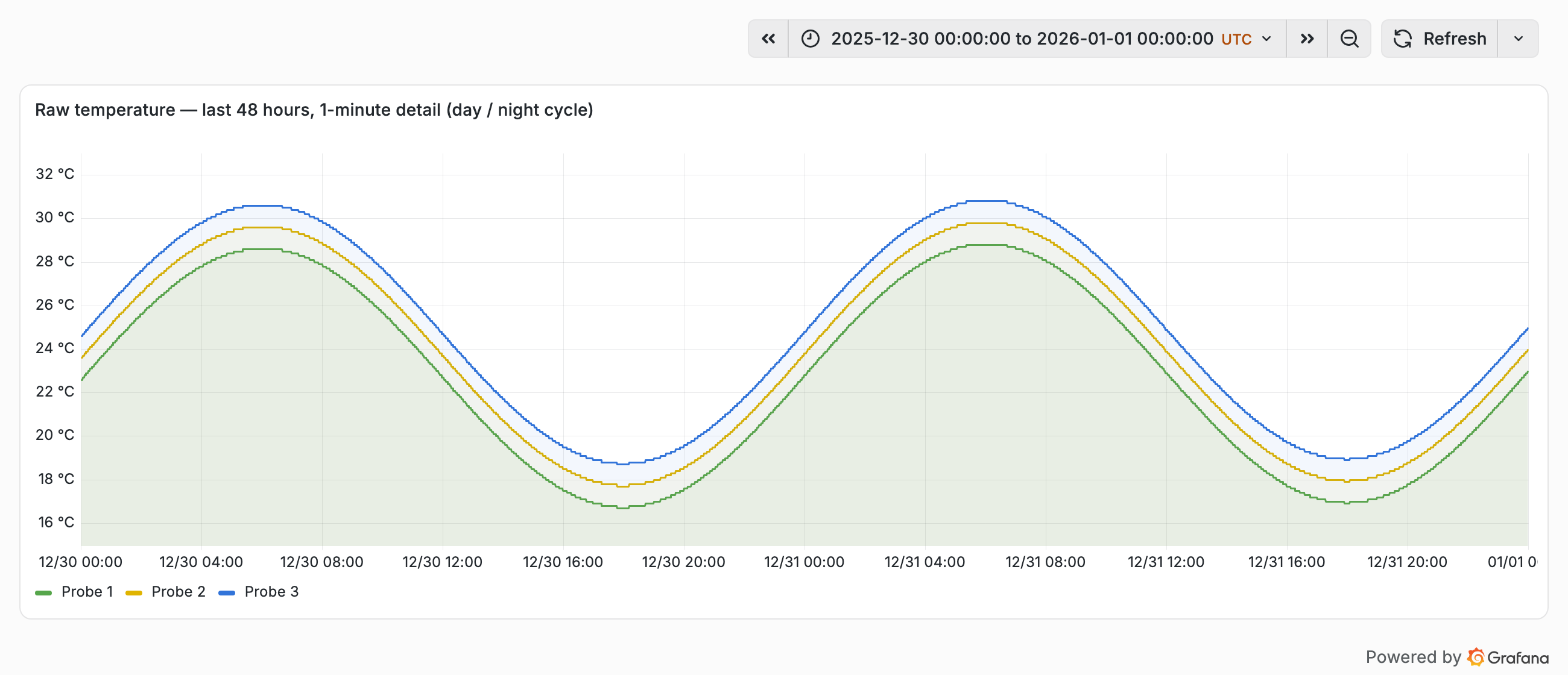
Zoom into the last 48 hours of raw one-minute data and the day/night cycle riding under that season appears — you can even see the 0.1 °C stair-steps of the rounded sensor values:
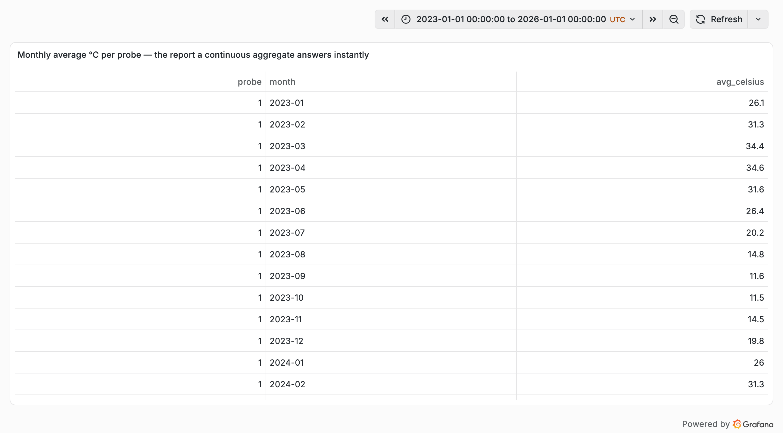
And the report itself — monthly average per probe, served from the continuous aggregate — is a table panel that returns the instant it's opened:
Conclusion
For a plant historian, the trade is clear and it's a good one. You pay about a third more on ingest, and a little index overhead on disk before compression. In return:
- The long data plane stops being the disk problem. Three years of raw minute-data went from 2.9 GB of plain Postgres to under 1 GB compressed, and stayed fully queryable. On real, flatter plant signals the saving is larger still.
- Reports over years become instant. The monthly-average-over-three-years query — the one everyone actually asks — dropped from five seconds to eight milliseconds through a continuous aggregate. That's the difference between a report you dread and a dashboard that's always warm.
- Recent-window queries are effectively free. Time partitioning gave a ~1300× speed-up on "last 24 hours" with zero extra tuning.
Would I run it in a plant? For anything that has to answer questions over long time spans — energy reporting, OEE trending, regulatory history — yes, without hesitation. It's PostgreSQL, so it drops into a stack your team already knows, under a UNS or behind Grafana, on-prem when the plant demands it. If your only need is "show me the live value" and you never look back more than an hour, a plain table or even a flat file is fine — you won't feel any of this. The moment history matters, the hypertable is the better place to keep it.
Newsletter
New essays, by email.
SCADA, cloud, AI, and the plant floor — a short email when something new is published. No noise, unsubscribe anytime.