Concluded·1 Aug 2026 · 5 min read
ClickHouse against TimescaleDB, ten million readings, same file into both
ClickHouse 24.8 · TimescaleDB pg17 · Docker Compose · Proxmox LXC
Ten million readings, two engines, one box. The rule I set was that both had to be loaded from the same file, because two separate loading scripts would have meant measuring my own code rather than the databases.
The rig
| Host | Proxmox LXC, 6 vCPU, 9 GB RAM, both engines co-resident |
| ClickHouse | 24.8, MergeTree ORDER BY (tag, ts) |
| TimescaleDB | pg17, hypertable on ts, 1.5 GB shared buffers |
| Dataset | 10,000,000 rows · 1,000 tags · 10,000 samples · 2h 46m |
The data is the output of the ten-million-point generator — six signal kinds shaped like plant behaviour. That choice is load-bearing rather than decorative: the same volume of uniform random numbers compresses about five times worse, so a benchmark built on noise would have made both engines look far more expensive to run than they are.
A bug I had to fix first
The file generator wrote ten million rows and reported ten million rows, and was
wrong. It held its position in the tag loop as a for variable, and resumed
from a backpressure event by re-entering the function — which quietly reset that
variable to zero, duplicating rows within a sample and skipping the rest of it.
The row count was exactly right, which is what made it hard to see. What gave it
away was the last timestamp in the file: 1,000 tags × 10,000 samples should end
at 02:46:39 and it ended at 01:23:20. Fixed by holding the position outside the
loop, and verified by counting distinct (ts, tag) pairs — 10,000,000 for
10,000,000 rows.
Worth stating plainly: had I not checked, every number below would have been computed over a dataset with duplicate rows, and duplicates compress beautifully. The compression figures would have been flattering nonsense.
Loading
| Time | Rows/sec | |
|---|---|---|
| ClickHouse | 3.75 s | 2,666,667 |
| TimescaleDB | 41.2 s | 242,600 |
LOADING THE SAME 10,000,000-ROW FILE
11× apart, on the identical file.
Storage
| On disk | Bytes per reading | |
|---|---|---|
| TimescaleDB, uncompressed | 698 MB | 73.2 |
| ClickHouse, default codec (LZ4) | 41.81 MiB | 4.38 |
| TimescaleDB, compressed | 16 MB | 1.68 |
| ClickHouse, tuned codecs | 6.35 MiB | 0.67 |
WHAT TEN MILLION READINGS COST TO KEEP
ClickHouse's default came out worse than compressed TimescaleDB, which was not
what I expected from a column store with that reputation. The default codec is
LZ4, chosen for speed rather than size. Giving the table the encodings that suit
time-series data — DoubleDelta on the timestamp, Gorilla on the float, both
inside ZSTD(3) — changed it completely:
CREATE TABLE points_zstd (
  ts    DateTime64(3) CODEC(DoubleDelta, ZSTD(3)),
  tag   LowCardinality(String),
  kind  LowCardinality(String),
  value Float64       CODEC(Gorilla, ZSTD(3))
) ENGINE = MergeTree ORDER BY (tag, ts);
Rewriting the same ten million rows into it took 2.3 seconds.
CHANGING THAT ONE SETTING — WHAT MOVES
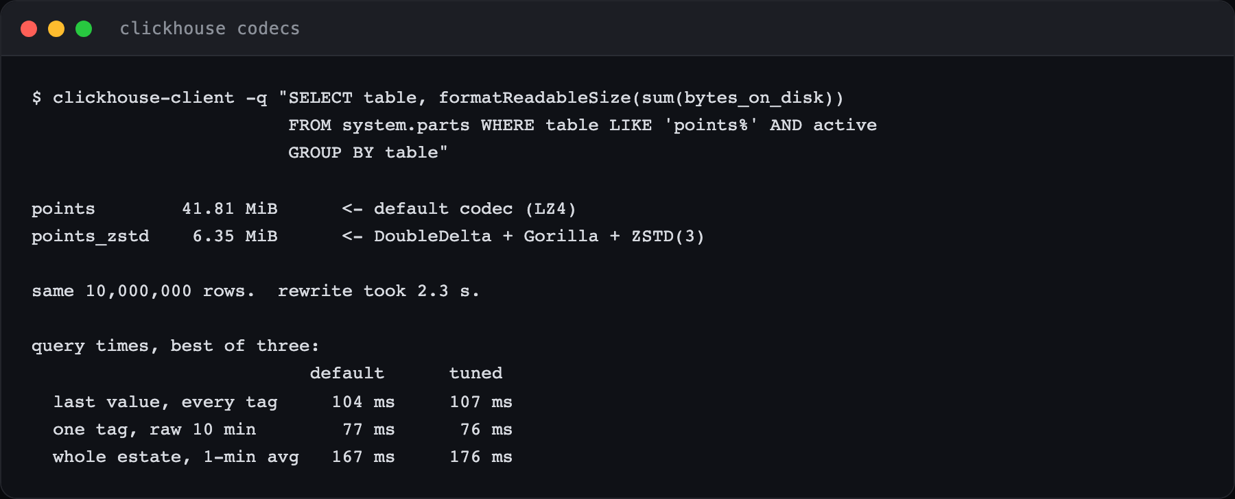
6.6× less disk, and every query landed within a few milliseconds of where it was. This is not a speed-versus-size decision to weigh up. It is a default that does not suit the job, and it is invisible unless you go looking.
Queries
Best of three runs, warm cache, milliseconds. These are the shapes a historian gets asked, not synthetic ones.
| Query | ClickHouse | CH tuned | Timescale raw | Timescale compressed |
|---|---|---|---|---|
| last value for every tag | 104 | 107 | 11,204 | 508 |
| one tag, raw 10-minute trace | 77 | 76 | 81 | 57 |
| one tag, 1-minute averages | 76 | 76 | 247 | 59 |
| whole estate, 1-minute averages | 167 | 176 | 1,202 | 1,955 |
| worst 20 vibration tags | 88 | 87 | 311 | 155 |
QUERY TIMES, BEST OF THREE, MILLISECONDS
| ClickHouse | ClickHouse, tuned | Timescale | Timescale, squeezed | |
|---|---|---|---|---|
| what is everything reading now | 104 | 107 | 11,204 | 508 |
| one instrument, last 10 min | 77 | 76 | 81 | 57 |
| one instrument, averaged | 76 | 76 | 247 | 59 |
| add up the whole site | 167 | 176 | 1,202 | 1,955 |
| worst 20 vibration readings | 88 | 87 | 311 | 155 |
The last-value query is brutal on an uncompressed hypertable. 11.2 seconds against 104 ms — 108× — for the single most routine question a control room asks. Compression takes it to 508 ms, usable, still 5× behind.
In fairness to TimescaleDB, this is a known pattern with known answers:
continuous aggregates maintaining a last-value table, or SkipScan on a
(tag, ts DESC) index. I measured the query somebody writes first, not the
query somebody writes after reading the tuning guide. Anyone deploying it in
anger would fix this, and it is worth knowing it needs fixing.
Single-tag reads go the other way. Compressed TimescaleDB beat ClickHouse on both — 57 ms against 77, and 59 ms against 76. Pulling one instrument's trend is what operators do dozens of times a shift, and on that workload the row-store with compression is genuinely faster.
Compression made one query slower. The whole-estate rollup went 1,202 ms → 1,955 ms after compressing. A query that touches every row has to decompress every row on the way past. Compression pays on selective reads and charges on full scans, and it is worth knowing which of those your dashboards actually do.
THE FOUR NUMBERS
Verdict
CHOOSING BY WORKLOAD, NOT BY BENCHMARK
ClickHouse for hard ingest, long retention, and questions that sweep the estate. Eleven times faster to load, two and a half times smaller than compressed Timescale once its codecs are set, and several times quicker on every aggregate that crosses tags.
TimescaleDB if the day-to-day is one instrument at a time, if Postgres is already in the building, or if anything downstream expects to speak SQL to an ordinary database. That last one is worth more than it looks on a benchmark page. Grafana, the reporting tool, the application written in 2019 and the colleague who already knows Postgres are all real costs on one side and real savings on the other.
An honest limit on all of this. Ten million readings is roughly three hours of a thousand-tag plant. Both engines are comfortable at that size, and at this scale the right way to choose is operational fit rather than milliseconds. The gap widens with volume, which is when the load and storage numbers start to decide it.
The one change worth making on Monday, whichever you run, is the codec setting.
The argument, without the measurements, is in the article.
Newsletter
New essays, by email.
SCADA, cloud, AI, and the plant floor — a short email when something new is published. No noise, unsubscribe anytime.